


Satellite Crop Monitoring: How to Spot Hidden Field Problems
Satellite monitoring helps agronomists detect crop variability, identify areas requiring inspection, and follow crop development across fields and growing seasons. Its agronomic value depends on choosing the appropriate satellite data, interpreting different indices correctly, and connecting detected anomalies to field measurements and timely decisions.
For large farms and organizations managing many growers, the challenge extends beyond producing vegetation maps. A monitoring system must recognize meaningful changes, prioritize them, and support consistent agronomic follow-up.
This practical guide compares satellite technologies and vegetation indices, explains the limitations of remote sensing, and uses actual field observations to show why combining indices is more informative than relying on NDVI alone.
What to compare in satellite crop monitoring
The most useful comparison considers the agronomic decision the imagery is expected to support. A service with higher-resolution maps is not automatically better if images are too infrequent, arrive too late, or cannot be interpreted in the context of crop development.
| Criterion | What it means for field decisions |
|---|---|
| Spatial resolution | Determines the scale of variation that can potentially be identified, subject to canopy cover and image quality. |
| Spectral information | Determines which vegetation, moisture-related, and canopy characteristics can be investigated. |
| Temporal coverage | Determines how often usable images are available, including the effects of cloud cover. |
| Historical comparison | Helps distinguish persistent management zones from newly developing anomalies. |
| Crop-stage context | Helps distinguish normal development or senescence from unexpected changes. |
| Automated anomaly detection | Flags unusual changes and supports prioritization of field inspection. |
| Field verification and follow-up | Connects satellite observations to measurements, diagnosis, corrective actions, and monitoring of results. |
Comparing satellite data sources and resolution
Satellite sensors differ in spatial resolution, spectral bands, acquisition frequency, and sensitivity to weather conditions. A combination of sources can improve monitoring continuity and provide complementary information.
| Source | Typical characteristics | Practical applications and limitations |
|---|---|---|
| Sentinel-2 optical imagery | 10 m, 20 m, and 60 m bands; nominal five-day revisit for the standard two-satellite configuration | Crop vigor, chlorophyll-related indices, canopy moisture-related indices, and historical comparisons. Usable observations are reduced by clouds. |
| Landsat 8/9 optical and thermal imagery | 30 m multispectral imagery; thermal data with coarser native resolution; nominal eight-day combined revisit | Long-term vegetation trends and surface-temperature information. Small anomalies can be mixed within pixels. |
| Commercial high-resolution optical imagery | Meter-scale resolution, depending on provider and product | Smaller fields and localized management patterns. Cost, acquisition availability, and cloud cover need evaluation. |
| Satellite synthetic aperture radar (SAR) | Microwave observations, including acquisitions through clouds and at night | Additional information about crop structure and surface conditions. Radar response is affected by canopy geometry, soil moisture, viewing geometry, and processing methods. |
Spatial resolution is the ground dimension represented by a pixel, not a guarantee that every object of that size will be detected. At 10 m resolution, one pixel covers approximately 100 m². A small irrigation fault affecting several plants may be diluted by the surrounding healthy canopy, while a broad irrigation-sector problem may be visible.
The effective resolution also depends on the bands used to calculate an index. For example, Sentinel-2 NDVI can use 10 m red and near-infrared bands, whereas a common Sentinel-2 NDMI calculation uses a 20 m shortwave-infrared band. An NDMI map displayed on a 10 m grid does not necessarily contain independent 10 m information.
Acquisition frequency must also be separated from usable-image frequency. Optical satellites may pass over a field on schedule but produce images obscured by clouds or affected by shadows. Combining suitable satellite sources can improve coverage, although measurements from different sensors should not automatically be treated as interchangeable.
Comparing vegetation indices
Different indices respond to different aspects of a crop canopy. Each is useful for particular questions, but none establishes the cause of a field problem without supporting evidence.
| Index | What it reflects | Useful applications | Important limitation |
|---|---|---|---|
| NDVI – Normalized Difference Vegetation Index | Green vegetation cover and vigor | Crop establishment, development, broad vigor differences | Can saturate in dense canopies and remain high despite some kinds of stress or lodging. |
| EVI – Enhanced Vegetation Index | Vegetation signal with adjustments for canopy background and some atmospheric influences | Tracking vigorous vegetation and seasonal development | Still requires comparable acquisition conditions and crop-stage interpretation. |
| NDRE – Normalized Difference Red Edge Index | Chlorophyll-related spectral variability | Identifying canopy differences that may warrant nutritional investigation | Does not independently establish nitrogen deficiency. |
| NDMI – Normalized Difference Moisture Index | Near-infrared and shortwave-infrared response associated with canopy water content | Identifying moisture-related canopy differences and their progression | Does not directly measure soil water content, plant water potential, or irrigation requirement. |
| SAVI – Soil-Adjusted Vegetation Index | Vegetation signal adjusted for soil background | Early growth and partially covered soil | Depends on the suitability of the soil-adjustment assumptions. |
| Radar Vegetation Index (RVI) | Radar backscatter properties influenced by vegetation structure and scattering | Complementary observation of crop structure, including anomalies associated with lodging | Cannot uniquely diagnose lodging; responses vary with radar configuration, moisture, and canopy structure. |
NDVI = (NIR – Red) / (NIR + Red)
NDMI = (NIR – SWIR) / (NIR + SWIR)
Here, NIR is near-infrared reflectance and SWIR is shortwave-infrared reflectance. The displayed values and their interpretation depend on the sensor bands and processing method. RVI calculations also depend on the radar polarization data and algorithm, so thresholds should not be transferred between products without validation.
Field example: Barley with high NDVI, moisture-related stress signals, and lodging
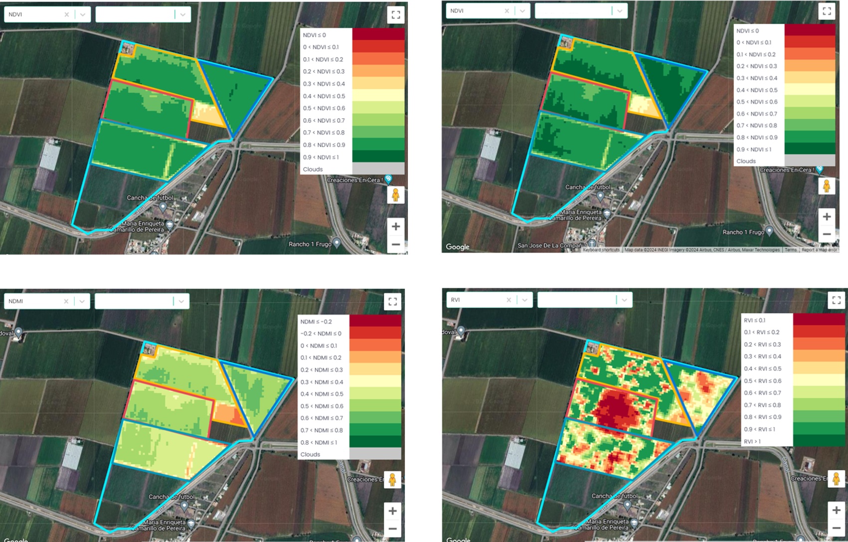
A barley field monitored with yieldsApp illustrates the benefit of comparing several indices. In the images from late February and early March 2024, NDVI was generally high across much of the crop, indicating a developed green canopy. Viewed alone, this could suggest relatively uniform crop vigor.
However, the NDMI map from March 4 showed substantially lower values in parts of the field, despite the high NDVI recorded on the same date. These areas raised a water-stress concern that the NDVI map did not make equally apparent. Low NDMI is consistent with changes in canopy water-related properties, but it is not sufficient by itself to confirm inadequate root-zone water supply. Verification would require soil and crop water-status observations and review of irrigation and weather conditions.
The radar vegetation index (RVI) map from March 6 showed additional spatial anomalies, including a prominent red area within the field. Field photographs showed visible barley lodging, providing ground evidence of a structural problem. In this example, radar information helped highlight an area associated with lodged plants, while NDVI continued to indicate substantial green vegetation.
Why lodging can be missed by NDVI
Lodging occurs when cereal stems or root systems fail to keep plants upright. Lodged barley can remain green for some time, so an index primarily responding to green vegetation may not fully represent the extent of canopy displacement or harvesting difficulties.
Radar measurements respond to scattering from the vegetation canopy and underlying surface. Changes in stem orientation and canopy geometry can alter radar backscatter and derived indices. Nevertheless, radar anomalies are not specific to lodging: soil or canopy moisture, incidence angle, and processing artifacts can produce changes as well.
The combination of satellite indices and the field photograph therefore supports the lodging interpretation in this case. It does not establish a universal RVI threshold for lodging detection.
Field example: NDMI reveals moisture-related variability where NDVI remains relatively high
Another field monitored on March 27, 2024, illustrates a similar difference between vegetation vigor and canopy moisture-related characteristics. The NDVI image shows generally moderate-to-high values across the circular field, while the NDMI map displays markedly lower values, including extensive orange and red zones.
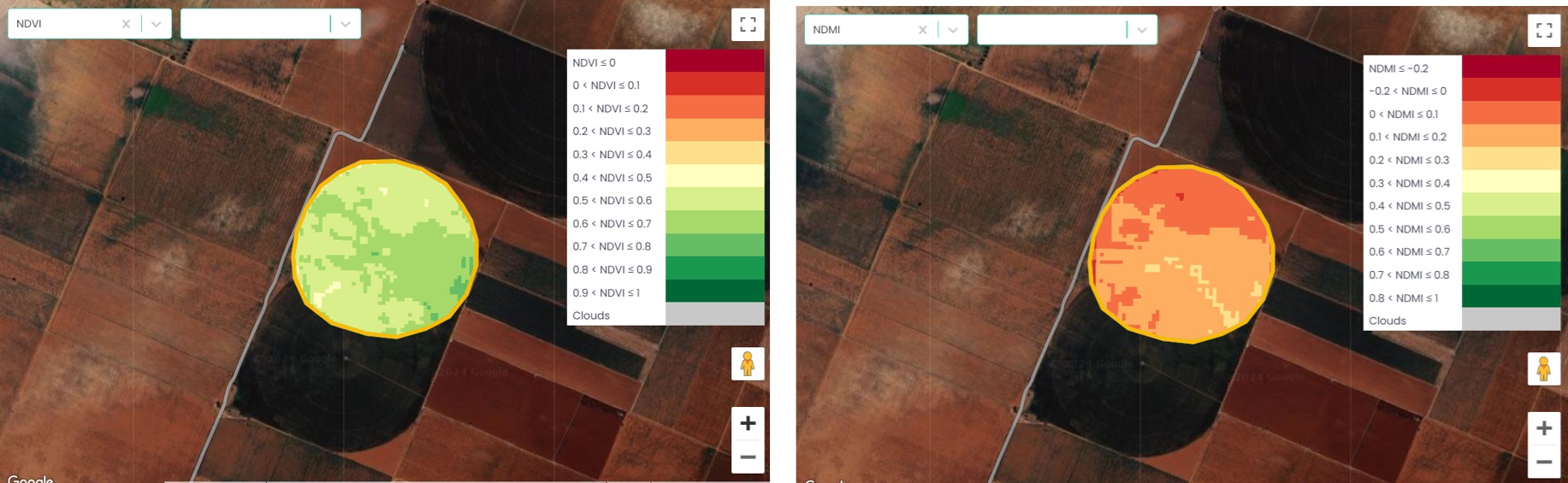
This comparison can help prioritize investigation of potential water stress. A useful field assessment would include:
- Soil water measurements at depths representing the active root zone, interpreted against field capacity, depletion, and soil texture.
- Recent irrigation amounts, distribution uniformity, and any system faults.
- Weather conditions and estimated crop evapotranspiration (ETc).
- Crop development stage, rooting conditions, and visible symptoms.
- Where appropriate, direct plant water-status measurements or other independent observations.
NDMI should not be converted directly into irrigation volume or a universal water-stress category. The interpretation is stronger when changes are compared with historical images, similar crop stages, and actual field conditions.
How to identify meaningful anomalies
An isolated low-value pixel may result from soil background, a field boundary, shadows, mixed land cover, or processing noise. Other differences may reflect persistent soil variation or normal crop development rather than a new management problem.
Three comparisons are especially useful:
- Within-field comparison: Compare anomalous zones with other parts of the same field, while accounting for management blocks and soil differences.
- Time-series comparison: Check whether a change is newly emerging, stable, expanding, or recovering across valid images.
- Historical comparison: Examine whether the same zone shows recurrent problems in comparable crops and phenological stages.
Automated anomaly detection can reduce the need for constant manual map review. In yieldsApp, satellite data from a combination of sources is used to monitor fields and identify anomalies automatically. These results help agronomic teams focus attention on fields that require further examination.
There is no reliable universal NDVI, NDMI, or RVI alert threshold for all crops. Alert rules should consider index-specific behavior, image quality, anomaly size, temporal persistence, crop stage, and the possible cost of a delayed response. A single observation may justify immediate inspection if the suspected problem is severe and time-sensitive.
Field verification: From an anomaly to an agronomic decision
Satellite observations should lead to a targeted inspection protocol that reflects the likely causes of the anomaly. Field technicians should examine both the affected area and a representative reference zone using comparable methods.
| Observed concern | What to verify in the field |
|---|---|
| Possible water stress | Soil water profile, irrigation timing and volume, distribution uniformity, rooting depth, plant water status, ETc. |
| Possible lodging | Percentage of area lodged, stem inclination and severity, growth stage, wind/rain history, crop stand density, harvest implications. |
| Reduced canopy vigor | Plant population, rooting restrictions, nutrient supply, pest and disease symptoms, compaction, waterlogging, and management history. |
| Suspected nutrient deficiency | Fertilization history, soil and tissue analyses where justified, crop stage, root condition, moisture limitations. |
| Possible salinity | Soil EC using a documented extraction method, irrigation-water quality, drainage, and distribution of salts in the root zone. |
Sampling must be suited to the spatial pattern. A large heterogeneous anomaly may require multiple sampling points rather than a single measurement. Document sampling locations, dates, methods, photographs, and findings. If the evidence is inconclusive, additional diagnostics may be more appropriate than an immediate treatment recommendation.
From satellite monitoring to coordinated field execution
For organizations managing many fields or growers, the value of monitoring depends on operational follow-through. A consistent process includes five steps:
- Detect: Identify abnormal spatial or temporal patterns, automatically where supported, and record the observation date and affected zone.
- Prioritize: Evaluate crop stage, anomaly progression, weather, management history, and consequences of delay.
- Verify: Assign a field inspection, collect relevant measurements, and establish the likely cause.
- Act: Document the agronomic recommendation, responsible person, and required intervention.
- Follow up: Confirm completion and evaluate field response with direct measurements and subsequent imagery.
This framework also supports consistency across regions. When agronomists and field technicians use common inspection procedures and record their actions, managers can track unresolved issues, compare outcomes, and improve the quality of agronomic execution across distributed farming systems.
yieldsApp supports this operational approach by combining satellite monitoring and automated anomaly identification with the broader agronomic context required for field-level decisions. Linking observations to agronomic workflows helps organizations coordinate, standardize, monitor, and scale execution across their grower networks.
Choosing a satellite monitoring approach
Different production systems require different priorities. Large cereal-growing operations may benefit from frequent broad-area monitoring and reliable time-series comparisons. Orchards and fragmented high-value cropping systems may need finer spatial detail and greater attention to mixed pixels. Organizations managing thousands of growers need repeatable alert review and field-verification procedures that work across many teams.
Before committing to a monitoring service, evaluate it against documented field events. For example, test whether the system highlighted known irrigation non-uniformity, lodging, persistent salinity zones, or uneven establishment, and whether those observations were available early enough to affect management.
When interpreting recurring problems, crop-specific irrigation management, soil and tissue analyses, crop physiology, and practical agronomic training are important complements to satellite data. Cropaia’s agronomy training resources support this field-specific interpretation.
Conclusion
Satellite monitoring is most useful when multiple sources and indices are interpreted together, in the context of crop physiology and field management. The barley examples show why high NDVI alone cannot rule out moisture-related stress or lodging: NDMI and radar measurements can reveal different aspects of the same crop.
Reliable decisions require verification. Combining automated anomaly detection, relevant field measurements, clear responsibilities, and documented follow-up enables farms and grower networks to turn satellite observations into timely and traceable agronomic action.










About Post Author
